Tonton Sekarang Tutorial ini memiliki kursus video terkait yang dibuat oleh tim Real Python. Tonton bersama dengan tutorial tertulis untuk memperdalam pemahaman Anda:Membaca dan Menulis File Dengan Pandas
Panda adalah paket Python yang kuat dan fleksibel yang memungkinkan Anda bekerja dengan data berlabel dan deret waktu. Ini juga menyediakan metode statistik, memungkinkan merencanakan, dan banyak lagi. Salah satu fitur penting Pandas adalah kemampuannya untuk menulis dan membaca Excel, CSV, dan banyak jenis file lainnya. Fungsi seperti read_csv() Pandas metode memungkinkan Anda untuk bekerja dengan file secara efektif. Anda dapat menggunakannya untuk menyimpan data dan label dari objek Pandas ke file dan memuatnya nanti sebagai Series Pandas atau DataFrame contoh.
Dalam tutorial ini, Anda akan mempelajari:
- Apa Alat Pandas IO API adalah
- Cara membaca dan menulis data ke dan dari file
- Cara bekerja dengan berbagai format file
- Cara bekerja dengan data besar efisien
Mari mulai membaca dan menulis file!
Bonus Gratis: 5 Thoughts On Python Mastery, kursus gratis untuk developer Python yang menunjukkan peta jalan dan pola pikir yang Anda perlukan untuk meningkatkan keterampilan Python Anda.
Menginstal Panda
Kode dalam tutorial ini dijalankan dengan CPython 3.7.4 dan Pandas 0.25.1. Akan bermanfaat untuk memastikan Anda memiliki versi terbaru Python dan Pandas di mesin Anda. Anda mungkin ingin membuat lingkungan virtual baru dan menginstal dependensi untuk tutorial ini.
Pertama, Anda memerlukan perpustakaan Pandas. Kamu mungkin sudah menginstalnya. Jika tidak, Anda dapat menginstalnya dengan pip:
$ pip install pandas
Setelah proses penginstalan selesai, Anda seharusnya sudah menginstal Pandas dan siap.
Anaconda adalah distribusi Python luar biasa yang hadir dengan Python, banyak paket berguna seperti Pandas, dan manajer paket dan lingkungan bernama Conda. Untuk mempelajari lebih lanjut tentang Anaconda, lihat Menyiapkan Python untuk Pembelajaran Mesin di Windows.
Jika Anda tidak memiliki Panda di lingkungan virtual Anda, Anda dapat menginstalnya dengan Conda:
$ conda install pandas
Conda sangat kuat karena mengelola dependensi dan versinya. Untuk mempelajari lebih lanjut tentang bekerja dengan Conda, Anda dapat melihat dokumentasi resmi.
Menyiapkan Data
Dalam tutorial ini, Anda akan menggunakan data yang terkait dengan 20 negara. Berikut ini ikhtisar data dan sumber yang akan Anda gunakan:
-
Negara dilambangkan dengan nama negara. Setiap negara berada dalam daftar 10 teratas baik untuk populasi, wilayah, atau produk domestik bruto (PDB). Label baris untuk kumpulan data adalah kode negara tiga huruf yang ditentukan dalam ISO 3166-1. Label kolom untuk kumpulan data adalah
COUNTRY. -
Populasi dinyatakan dalam jutaan. Data berasal dari daftar negara dan dependensi berdasarkan populasi di Wikipedia. Label kolom untuk kumpulan data adalah
POP. -
Wilayah dinyatakan dalam ribuan kilometer persegi. Data berasal dari daftar negara dan dependensi berdasarkan wilayah di Wikipedia. Label kolom untuk kumpulan data adalah
AREA. -
Produk domestik bruto dinyatakan dalam jutaan dolar AS, menurut data Perserikatan Bangsa-Bangsa untuk tahun 2017. Anda dapat menemukan data ini dalam daftar negara menurut PDB nominal di Wikipedia. Label kolom untuk kumpulan data adalah
GDP. -
Benua adalah Afrika, Asia, Oseania, Eropa, Amerika Utara, atau Amerika Selatan. Anda juga dapat menemukan informasi ini di Wikipedia. Label kolom untuk kumpulan data adalah
CONT. -
Hari kemerdekaan adalah tanggal yang memperingati kemerdekaan suatu bangsa. Data tersebut berasal dari daftar hari kemerdekaan nasional di Wikipedia. Tanggal ditampilkan dalam format ISO 8601. Empat digit pertama menunjukkan tahun, dua angka berikutnya adalah bulan, dan dua angka terakhir menunjukkan hari dalam sebulan. Label kolom untuk kumpulan data adalah
IND_DAY.
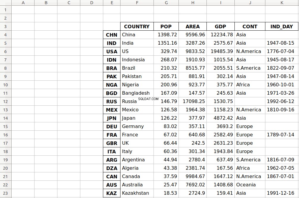
Berikut tampilan data sebagai tabel:
| NEGARA | POP | AREA | PDB | LANJUTKAN | HARI_IND | |
|---|---|---|---|---|---|---|
| CHN | Cina | 1398,72 | 9596,96 | 12234,78 | Asia | |
| IND | India | 1351.16 | 3287,26 | 2575,67 | Asia | 1947-08-15 |
| AS | AS | 329,74 | 9833.52 | 19485.39 | N.Amerika | 1776-07-04 |
| IDN | Indonesia | 268.07 | 1910,93 | 1015,54 | Asia | 17-08-45 |
| BRA | Brasil | 210.32 | 8515,77 | 2055.51 | Amerika Serikat | 1822-09-07 |
| PAK | Pakistan | 205.71 | 881.91 | 302.14 | Asia | 14-08-47 |
| NGA | Nigeria | 200,96 | 923,77 | 375,77 | Afrika | 19-10-01 |
| BGD | Bangladesh | 167.09 | 147,57 | 245.63 | Asia | 26-03-71 |
| RUS | Rusia | 146,79 | 17098,25 | 1530,75 | 2012-06-12 | |
| MEX | Meksiko | 126,58 | 1964.38 | 1158,23 | N.Amerika | 1810-09-16 |
| JPN | Jepang | 126.22 | 377,97 | 4872.42 | Asia | |
| DEU | Jerman | 83,02 | 357.11 | 3693.20 | Eropa | |
| FRA | Prancis | 67,02 | 640.68 | 2582,49 | Eropa | 1789-07-14 |
| GBR | Inggris Raya | 66,44 | 242,50 | 2631.23 | Eropa | |
| ITA | Italia | 60,36 | 301,34 | 1943,84 | Eropa | |
| ARG | Argentina | 44,94 | 2780.40 | 637.49 | Amerika Serikat | 1816-07-09 |
| DZA | Aljazair | 43,38 | 2381,74 | 167,56 | Afrika | 06-07-05 |
| BISA | Kanada | 37,59 | 9984,67 | 1647.12 | N.Amerika | 1867-07-01 |
| AUS | Australia | 25,47 | 7692.02 | 1408,68 | Oseania | |
| KAZ | Kazakhstan | 18,53 | 2724.90 | 159,41 | Asia | 1991-12-16 |
Anda mungkin memperhatikan bahwa beberapa data hilang. Misalnya, benua untuk Rusia tidak ditentukan karena tersebar di Eropa dan Asia. Ada juga beberapa hari kemerdekaan yang hilang karena sumber data menghilangkannya.
Anda dapat mengatur data ini dengan Python menggunakan kamus bersarang:
data = {
    'CHN': {'COUNTRY': 'China', 'POP': 1_398.72, 'AREA': 9_596.96,
            'GDP': 12_234.78, 'CONT': 'Asia'},
    'IND': {'COUNTRY': 'India', 'POP': 1_351.16, 'AREA': 3_287.26,
            'GDP': 2_575.67, 'CONT': 'Asia', 'IND_DAY': '1947-08-15'},
    'USA': {'COUNTRY': 'US', 'POP': 329.74, 'AREA': 9_833.52,
            'GDP': 19_485.39, 'CONT': 'N.America',
            'IND_DAY': '1776-07-04'},
    'IDN': {'COUNTRY': 'Indonesia', 'POP': 268.07, 'AREA': 1_910.93,
            'GDP': 1_015.54, 'CONT': 'Asia', 'IND_DAY': '1945-08-17'},
    'BRA': {'COUNTRY': 'Brazil', 'POP': 210.32, 'AREA': 8_515.77,
            'GDP': 2_055.51, 'CONT': 'S.America', 'IND_DAY': '1822-09-07'},
    'PAK': {'COUNTRY': 'Pakistan', 'POP': 205.71, 'AREA': 881.91,
            'GDP': 302.14, 'CONT': 'Asia', 'IND_DAY': '1947-08-14'},
    'NGA': {'COUNTRY': 'Nigeria', 'POP': 200.96, 'AREA': 923.77,
            'GDP': 375.77, 'CONT': 'Africa', 'IND_DAY': '1960-10-01'},
    'BGD': {'COUNTRY': 'Bangladesh', 'POP': 167.09, 'AREA': 147.57,
            'GDP': 245.63, 'CONT': 'Asia', 'IND_DAY': '1971-03-26'},
    'RUS': {'COUNTRY': 'Russia', 'POP': 146.79, 'AREA': 17_098.25,
            'GDP': 1_530.75, 'IND_DAY': '1992-06-12'},
    'MEX': {'COUNTRY': 'Mexico', 'POP': 126.58, 'AREA': 1_964.38,
            'GDP': 1_158.23, 'CONT': 'N.America', 'IND_DAY': '1810-09-16'},
    'JPN': {'COUNTRY': 'Japan', 'POP': 126.22, 'AREA': 377.97,
            'GDP': 4_872.42, 'CONT': 'Asia'},
    'DEU': {'COUNTRY': 'Germany', 'POP': 83.02, 'AREA': 357.11,
            'GDP': 3_693.20, 'CONT': 'Europe'},
    'FRA': {'COUNTRY': 'France', 'POP': 67.02, 'AREA': 640.68,
            'GDP': 2_582.49, 'CONT': 'Europe', 'IND_DAY': '1789-07-14'},
    'GBR': {'COUNTRY': 'UK', 'POP': 66.44, 'AREA': 242.50,
            'GDP': 2_631.23, 'CONT': 'Europe'},
    'ITA': {'COUNTRY': 'Italy', 'POP': 60.36, 'AREA': 301.34,
            'GDP': 1_943.84, 'CONT': 'Europe'},
    'ARG': {'COUNTRY': 'Argentina', 'POP': 44.94, 'AREA': 2_780.40,
            'GDP': 637.49, 'CONT': 'S.America', 'IND_DAY': '1816-07-09'},
    'DZA': {'COUNTRY': 'Algeria', 'POP': 43.38, 'AREA': 2_381.74,
            'GDP': 167.56, 'CONT': 'Africa', 'IND_DAY': '1962-07-05'},
    'CAN': {'COUNTRY': 'Canada', 'POP': 37.59, 'AREA': 9_984.67,
            'GDP': 1_647.12, 'CONT': 'N.America', 'IND_DAY': '1867-07-01'},
    'AUS': {'COUNTRY': 'Australia', 'POP': 25.47, 'AREA': 7_692.02,
            'GDP': 1_408.68, 'CONT': 'Oceania'},
    'KAZ': {'COUNTRY': 'Kazakhstan', 'POP': 18.53, 'AREA': 2_724.90,
            'GDP': 159.41, 'CONT': 'Asia', 'IND_DAY': '1991-12-16'}
}

columns = ('COUNTRY', 'POP', 'AREA', 'GDP', 'CONT', 'IND_DAY')
Setiap baris tabel ditulis sebagai kamus bagian dalam yang kuncinya adalah nama kolom dan nilainya adalah data yang sesuai. Kamus ini kemudian dikumpulkan sebagai nilai di data luar kamus. Kunci yang sesuai untuk data adalah kode negara tiga huruf.
Anda dapat menggunakan data ini untuk membuat instance dari DataFrame Panda Pandas . Pertama, Anda perlu mengimpor Panda:
>>> import pandas as pd
Sekarang setelah Anda mengimpor Panda, Anda dapat menggunakan DataFrame konstruktor dan data untuk membuat DataFrame objek.
data diatur sedemikian rupa sehingga kode negara sesuai dengan kolom. Anda dapat membalikkan baris dan kolom dari DataFrame dengan properti .T :
>>> df = pd.DataFrame(data=data).T
>>> df
        COUNTRY      POP     AREA      GDP       CONT     IND_DAY
CHN       China  1398.72  9596.96  12234.8       Asia         NaN
IND       India  1351.16  3287.26  2575.67       Asia  1947-08-15
USA          US   329.74  9833.52  19485.4  N.America  1776-07-04
IDN   Indonesia   268.07  1910.93  1015.54       Asia  1945-08-17
BRA      Brazil   210.32  8515.77  2055.51  S.America  1822-09-07
PAK    Pakistan   205.71   881.91   302.14       Asia  1947-08-14
NGA     Nigeria   200.96   923.77   375.77     Africa  1960-10-01
BGD  Bangladesh   167.09   147.57   245.63       Asia  1971-03-26
RUS      Russia   146.79  17098.2  1530.75        NaN  1992-06-12
MEX      Mexico   126.58  1964.38  1158.23  N.America  1810-09-16
JPN       Japan   126.22   377.97  4872.42       Asia         NaN
DEU     Germany    83.02   357.11   3693.2     Europe         NaN
FRA      France    67.02   640.68  2582.49     Europe  1789-07-14
GBR          UK    66.44    242.5  2631.23     Europe         NaN
ITA       Italy    60.36   301.34  1943.84     Europe         NaN
ARG   Argentina    44.94   2780.4   637.49  S.America  1816-07-09
DZA     Algeria    43.38  2381.74   167.56     Africa  1962-07-05
CAN      Canada    37.59  9984.67  1647.12  N.America  1867-07-01
AUS   Australia    25.47  7692.02  1408.68    Oceania         NaN
KAZ  Kazakhstan    18.53   2724.9   159.41       Asia  1991-12-16
Sekarang Anda memiliki DataFrame objek diisi dengan data tentang setiap negara.
Catatan: Anda dapat menggunakan .transpose() bukannya .T untuk membalikkan baris dan kolom kumpulan data Anda. Jika Anda menggunakan .transpose() , maka Anda dapat mengatur parameter opsional copy untuk menentukan apakah Anda ingin menyalin data yang mendasarinya. Perilaku default adalah False .
Versi Python yang lebih lama dari 3.6 tidak menjamin urutan kunci dalam kamus. Untuk memastikan urutan kolom dipertahankan untuk versi Python dan Panda yang lebih lama, Anda dapat menentukan index=columns :
>>> df = pd.DataFrame(data=data, index=columns).T
Sekarang setelah Anda menyiapkan data, Anda siap untuk mulai bekerja dengan file!
Menggunakan read_csv() Pandas dan .to_csv() Fungsi
File nilai yang dipisahkan koma (CSV) adalah file teks biasa dengan .csv ekstensi yang menyimpan data tabular. Ini adalah salah satu format file paling populer untuk menyimpan data dalam jumlah besar. Setiap baris file CSV mewakili satu baris tabel. Nilai di baris yang sama secara default dipisahkan dengan koma, tetapi Anda dapat mengubah pemisah menjadi titik koma, tab, spasi, atau karakter lain.
Menulis File CSV
Anda dapat menyimpan DataFrame Panda Anda sebagai file CSV dengan .to_csv() :
>>> df.to_csv('data.csv')
Itu dia! Anda telah membuat file data.csv di direktori kerja Anda saat ini. Anda dapat memperluas blok kode di bawah ini untuk melihat tampilan file CSV Anda:
,COUNTRY,POP,AREA,GDP,CONT,IND_DAY
CHN,China,1398.72,9596.96,12234.78,Asia,
IND,India,1351.16,3287.26,2575.67,Asia,1947-08-15
USA,US,329.74,9833.52,19485.39,N.America,1776-07-04
IDN,Indonesia,268.07,1910.93,1015.54,Asia,1945-08-17
BRA,Brazil,210.32,8515.77,2055.51,S.America,1822-09-07
PAK,Pakistan,205.71,881.91,302.14,Asia,1947-08-14
NGA,Nigeria,200.96,923.77,375.77,Africa,1960-10-01
BGD,Bangladesh,167.09,147.57,245.63,Asia,1971-03-26
RUS,Russia,146.79,17098.25,1530.75,,1992-06-12
MEX,Mexico,126.58,1964.38,1158.23,N.America,1810-09-16
JPN,Japan,126.22,377.97,4872.42,Asia,
DEU,Germany,83.02,357.11,3693.2,Europe,
FRA,France,67.02,640.68,2582.49,Europe,1789-07-14
GBR,UK,66.44,242.5,2631.23,Europe,
ITA,Italy,60.36,301.34,1943.84,Europe,
ARG,Argentina,44.94,2780.4,637.49,S.America,1816-07-09
DZA,Algeria,43.38,2381.74,167.56,Africa,1962-07-05
CAN,Canada,37.59,9984.67,1647.12,N.America,1867-07-01
AUS,Australia,25.47,7692.02,1408.68,Oceania,
KAZ,Kazakhstan,18.53,2724.9,159.41,Asia,1991-12-16
File teks ini berisi data yang dipisahkan dengan koma . Kolom pertama berisi label baris. Dalam beberapa kasus, Anda akan menganggapnya tidak relevan. Jika Anda tidak ingin menyimpannya, Anda dapat meneruskan argumen index=False ke .to_csv() .
Baca File CSV
Setelah data Anda disimpan dalam file CSV, Anda mungkin ingin memuat dan menggunakannya dari waktu ke waktu. Anda dapat melakukannya dengan read_csv() Panda Pandas fungsi:
>>> df = pd.read_csv('data.csv', index_col=0)
>>> df
        COUNTRY      POP      AREA       GDP       CONT     IND_DAY
CHN       China  1398.72   9596.96  12234.78       Asia         NaN
IND       India  1351.16   3287.26   2575.67       Asia  1947-08-15
USA          US   329.74   9833.52  19485.39  N.America  1776-07-04
IDN   Indonesia   268.07   1910.93   1015.54       Asia  1945-08-17
BRA      Brazil   210.32   8515.77   2055.51  S.America  1822-09-07
PAK    Pakistan   205.71    881.91    302.14       Asia  1947-08-14
NGA     Nigeria   200.96    923.77    375.77     Africa  1960-10-01
BGD  Bangladesh   167.09    147.57    245.63       Asia  1971-03-26
RUS      Russia   146.79  17098.25   1530.75        NaN  1992-06-12
MEX      Mexico   126.58   1964.38   1158.23  N.America  1810-09-16
JPN       Japan   126.22    377.97   4872.42       Asia         NaN
DEU     Germany    83.02    357.11   3693.20     Europe         NaN
FRA      France    67.02    640.68   2582.49     Europe  1789-07-14
GBR          UK    66.44    242.50   2631.23     Europe         NaN
ITA       Italy    60.36    301.34   1943.84     Europe         NaN
ARG   Argentina    44.94   2780.40    637.49  S.America  1816-07-09
DZA     Algeria    43.38   2381.74    167.56     Africa  1962-07-05
CAN      Canada    37.59   9984.67   1647.12  N.America  1867-07-01
AUS   Australia    25.47   7692.02   1408.68    Oceania         NaN
KAZ  Kazakhstan    18.53   2724.90    159.41       Asia  1991-12-16
Dalam hal ini, Panda read_csv() fungsi mengembalikan DataFrame baru dengan data dan label dari file data.csv , yang Anda tentukan dengan argumen pertama. String ini dapat berupa jalur apa pun yang valid, termasuk URL.
Parameter index_col menentukan kolom dari file CSV yang berisi label baris. Anda menetapkan indeks kolom berbasis nol untuk parameter ini. Anda harus menentukan nilai index_col saat file CSV berisi label baris untuk menghindari pemuatannya sebagai data.
Anda akan mempelajari lebih lanjut tentang menggunakan Pandas dengan file CSV nanti dalam tutorial ini. Anda juga dapat melihat Membaca dan Menulis File CSV dengan Python untuk melihat cara menangani file CSV dengan csv library Python bawaan juga.
Menggunakan Panda untuk Menulis dan Membaca File Excel
Microsoft Excel mungkin adalah perangkat lunak spreadsheet yang paling banyak digunakan. Sementara versi yang lebih lama menggunakan biner .xls file, Excel 2007 memperkenalkan .xlsx berbasis XML baru mengajukan. Anda dapat membaca dan menulis file Excel di Pandas, mirip dengan file CSV. Namun, Anda harus menginstal paket Python berikut terlebih dahulu:
- xlwt untuk menulis ke
.xlsfile - openpyxl atau XlsxWriter untuk menulis ke
.xlsxfile - xlrd untuk membaca file Excel
Anda dapat menginstalnya menggunakan pip dengan satu perintah:
$ pip install xlwt openpyxl xlsxwriter xlrd
Anda juga dapat menggunakan Conda:
$ conda install xlwt openpyxl xlsxwriter xlrd
Harap perhatikan bahwa Anda tidak perlu menginstal semua paket-paket ini. Misalnya, Anda tidak memerlukan openpyxl dan XlsxWriter. Jika Anda akan bekerja hanya dengan .xls file, maka Anda tidak memerlukannya! Namun, jika Anda ingin bekerja hanya dengan .xlsx file, maka Anda akan membutuhkan setidaknya satu dari mereka, tetapi tidak xlwt . Luangkan waktu untuk memutuskan paket mana yang tepat untuk proyek Anda.
Menulis File Excel
Setelah Anda menginstal paket tersebut, Anda dapat menyimpan DataFrame dalam file Excel dengan .to_excel() :
>>> df.to_excel('data.xlsx')
Argumen 'data.xlsx' mewakili file target dan, opsional, jalurnya. Pernyataan di atas harus membuat file data.xlsx di direktori kerja Anda saat ini. File itu akan terlihat seperti ini:
Kolom pertama file berisi label baris, sedangkan kolom lainnya menyimpan data.
Membaca File Excel
Anda dapat memuat data dari file Excel dengan read_excel() :
>>> df = pd.read_excel('data.xlsx', index_col=0)
>>> df
        COUNTRY      POP      AREA       GDP       CONT     IND_DAY
CHN       China  1398.72   9596.96  12234.78       Asia         NaN
IND       India  1351.16   3287.26   2575.67       Asia  1947-08-15
USA          US   329.74   9833.52  19485.39  N.America  1776-07-04
IDN   Indonesia   268.07   1910.93   1015.54       Asia  1945-08-17
BRA      Brazil   210.32   8515.77   2055.51  S.America  1822-09-07
PAK    Pakistan   205.71    881.91    302.14       Asia  1947-08-14
NGA     Nigeria   200.96    923.77    375.77     Africa  1960-10-01
BGD  Bangladesh   167.09    147.57    245.63       Asia  1971-03-26
RUS      Russia   146.79  17098.25   1530.75        NaN  1992-06-12
MEX      Mexico   126.58   1964.38   1158.23  N.America  1810-09-16
JPN       Japan   126.22    377.97   4872.42       Asia         NaN
DEU     Germany    83.02    357.11   3693.20     Europe         NaN
FRA      France    67.02    640.68   2582.49     Europe  1789-07-14
GBR          UK    66.44    242.50   2631.23     Europe         NaN
ITA       Italy    60.36    301.34   1943.84     Europe         NaN
ARG   Argentina    44.94   2780.40    637.49  S.America  1816-07-09
DZA     Algeria    43.38   2381.74    167.56     Africa  1962-07-05
CAN      Canada    37.59   9984.67   1647.12  N.America  1867-07-01
AUS   Australia    25.47   7692.02   1408.68    Oceania         NaN
KAZ  Kazakhstan    18.53   2724.90    159.41       Asia  1991-12-16
read_excel() mengembalikan DataFrame baru yang berisi nilai dari data.xlsx . Anda juga dapat menggunakan read_excel() dengan spreadsheet OpenDocument, atau .ods file.
Anda akan mempelajari lebih lanjut tentang bekerja dengan file Excel nanti dalam tutorial ini. Anda juga dapat melihat Menggunakan Panda untuk Membaca File Excel Besar dengan Python.
Memahami Pandas IO API
Alat Pandas IO adalah API yang memungkinkan Anda menyimpan konten Series dan DataFrame objek ke clipboard, objek, atau file dari berbagai jenis. Ini juga memungkinkan memuat data dari clipboard, objek, atau file.
Tulis File
Series dan DataFrame objek memiliki metode yang memungkinkan penulisan data dan label ke clipboard atau file. Mereka diberi nama dengan pola .to_<file-type>() , di mana <file-type> adalah jenis file target.
Anda telah mempelajari tentang .to_csv() dan .to_excel() , tetapi ada yang lain, termasuk:
.to_json().to_html().to_sql().to_pickle()
Masih ada lebih banyak jenis file yang dapat Anda gunakan untuk menulis, jadi daftar ini tidak lengkap.
Catatan: Untuk menemukan metode serupa, periksa dokumentasi resmi tentang serialisasi, IO, dan konversi yang terkait dengan Series dan DataFrame objek.
Metode ini memiliki parameter yang menentukan jalur file target tempat Anda menyimpan data dan label. Ini wajib dalam beberapa kasus dan opsional dalam kasus lain. Jika opsi ini tersedia dan Anda memilih untuk menghilangkannya, maka metode akan mengembalikan objek (seperti string atau iterable) dengan konten DataFrame contoh.
Parameter opsional compression memutuskan bagaimana mengompresi file dengan data dan label. Anda akan mempelajarinya lebih lanjut nanti. Ada beberapa parameter lain, tetapi sebagian besar khusus untuk satu atau beberapa metode. Anda tidak akan membahasnya secara mendetail di sini.
Baca File
Fungsi Pandas untuk membaca isi file diberi nama menggunakan pola .read_<file-type>() , di mana <file-type> menunjukkan jenis file yang akan dibaca. Anda telah melihat read_csv() Pandas dan read_excel() fungsi. Berikut beberapa lainnya:
read_json()read_html()read_sql()read_pickle()
Fungsi-fungsi ini memiliki parameter yang menentukan jalur file target. Itu bisa berupa string valid apa pun yang mewakili jalur, baik di mesin lokal atau di URL. Objek lain juga dapat diterima tergantung pada jenis file.
Parameter opsional compression menentukan jenis dekompresi yang akan digunakan untuk file terkompresi. Anda akan mempelajarinya nanti dalam tutorial ini. Ada parameter lain, tetapi mereka khusus untuk satu atau beberapa fungsi. Anda tidak akan membahasnya secara mendetail di sini.
Bekerja Dengan Berbagai Jenis File
Pustaka Pandas menawarkan berbagai kemungkinan untuk menyimpan data Anda ke file dan memuat data dari file. Di bagian ini, Anda akan mempelajari lebih lanjut tentang bekerja dengan file CSV dan Excel. Anda juga akan melihat cara menggunakan jenis file lain, seperti JSON, halaman web, database, dan file acar Python.
File CSV
Anda telah mempelajari cara membaca dan menulis file CSV. Sekarang mari kita gali lebih dalam ke detailnya. Saat Anda menggunakan .to_csv() untuk menyimpan DataFrame , Anda dapat memberikan argumen untuk parameter path_or_buf untuk menentukan jalur, nama, dan ekstensi file target.
path_or_buf adalah argumen pertama .to_csv() akan mendapatkan. Itu bisa berupa string apa pun yang mewakili jalur file yang valid yang menyertakan nama file dan ekstensinya. Anda telah melihat ini dalam contoh sebelumnya. Namun, jika Anda menghilangkan path_or_buf , lalu .to_csv() tidak akan membuat file apa pun. Sebagai gantinya, itu akan mengembalikan string yang sesuai:
>>> df = pd.DataFrame(data=data).T
>>> s = df.to_csv()
>>> print(s)
,COUNTRY,POP,AREA,GDP,CONT,IND_DAY
CHN,China,1398.72,9596.96,12234.78,Asia,
IND,India,1351.16,3287.26,2575.67,Asia,1947-08-15
USA,US,329.74,9833.52,19485.39,N.America,1776-07-04
IDN,Indonesia,268.07,1910.93,1015.54,Asia,1945-08-17
BRA,Brazil,210.32,8515.77,2055.51,S.America,1822-09-07
PAK,Pakistan,205.71,881.91,302.14,Asia,1947-08-14
NGA,Nigeria,200.96,923.77,375.77,Africa,1960-10-01
BGD,Bangladesh,167.09,147.57,245.63,Asia,1971-03-26
RUS,Russia,146.79,17098.25,1530.75,,1992-06-12
MEX,Mexico,126.58,1964.38,1158.23,N.America,1810-09-16
JPN,Japan,126.22,377.97,4872.42,Asia,
DEU,Germany,83.02,357.11,3693.2,Europe,
FRA,France,67.02,640.68,2582.49,Europe,1789-07-14
GBR,UK,66.44,242.5,2631.23,Europe,
ITA,Italy,60.36,301.34,1943.84,Europe,
ARG,Argentina,44.94,2780.4,637.49,S.America,1816-07-09
DZA,Algeria,43.38,2381.74,167.56,Africa,1962-07-05
CAN,Canada,37.59,9984.67,1647.12,N.America,1867-07-01
AUS,Australia,25.47,7692.02,1408.68,Oceania,
KAZ,Kazakhstan,18.53,2724.9,159.41,Asia,1991-12-16
Sekarang Anda memiliki string s alih-alih file CSV. Anda juga memiliki beberapa nilai yang hilang di DataFrame . Anda obyek. Misalnya, benua untuk Rusia dan hari-hari kemerdekaan untuk beberapa negara (Cina, Jepang, dan sebagainya) tidak tersedia. Dalam ilmu data dan pembelajaran mesin, Anda harus menangani nilai yang hilang dengan hati-hati. Panda unggul di sini! Secara default, Pandas menggunakan nilai NaN untuk menggantikan nilai yang hilang.
Catatan: nan , yang merupakan singkatan dari “bukan angka”, adalah nilai floating-point tertentu dalam Python.
Anda bisa mendapatkan nan nilai dengan salah satu fungsi berikut:
float('nan')math.nannumpy.nan
Benua yang sesuai dengan Rusia di df adalah nan :
>>> df.loc['RUS', 'CONT']
nan
Contoh ini menggunakan .loc[] untuk mendapatkan data dengan nama baris dan kolom yang ditentukan.
Saat Anda menyimpan DataFrame ke file CSV, string kosong ('' ) akan mewakili data yang hilang. Anda dapat melihat keduanya di file data.csv dan dalam string s . Jika Anda ingin mengubah perilaku ini, gunakan parameter opsional na_rep :
>>> df.to_csv('new-data.csv', na_rep='(missing)')
Kode ini menghasilkan file new-data.csv di mana nilai yang hilang bukan lagi string kosong. Anda dapat memperluas blok kode di bawah ini untuk melihat tampilan file ini:
,COUNTRY,POP,AREA,GDP,CONT,IND_DAY
CHN,China,1398.72,9596.96,12234.78,Asia,(missing)
IND,India,1351.16,3287.26,2575.67,Asia,1947-08-15
USA,US,329.74,9833.52,19485.39,N.America,1776-07-04
IDN,Indonesia,268.07,1910.93,1015.54,Asia,1945-08-17
BRA,Brazil,210.32,8515.77,2055.51,S.America,1822-09-07
PAK,Pakistan,205.71,881.91,302.14,Asia,1947-08-14
NGA,Nigeria,200.96,923.77,375.77,Africa,1960-10-01
BGD,Bangladesh,167.09,147.57,245.63,Asia,1971-03-26
RUS,Russia,146.79,17098.25,1530.75,(missing),1992-06-12
MEX,Mexico,126.58,1964.38,1158.23,N.America,1810-09-16
JPN,Japan,126.22,377.97,4872.42,Asia,(missing)
DEU,Germany,83.02,357.11,3693.2,Europe,(missing)
FRA,France,67.02,640.68,2582.49,Europe,1789-07-14
GBR,UK,66.44,242.5,2631.23,Europe,(missing)
ITA,Italy,60.36,301.34,1943.84,Europe,(missing)
ARG,Argentina,44.94,2780.4,637.49,S.America,1816-07-09
DZA,Algeria,43.38,2381.74,167.56,Africa,1962-07-05
CAN,Canada,37.59,9984.67,1647.12,N.America,1867-07-01
AUS,Australia,25.47,7692.02,1408.68,Oceania,(missing)
KAZ,Kazakhstan,18.53,2724.9,159.41,Asia,1991-12-16
Now, the string '(missing)' in the file corresponds to the nan values from df .
When Pandas reads files, it considers the empty string ('' ) and a few others as missing values by default:
'nan''-nan''NA''N/A''NaN''null'
If you don’t want this behavior, then you can pass keep_default_na=False to the Pandas read_csv() fungsi. To specify other labels for missing values, use the parameter na_values :
>>> pd.read_csv('new-data.csv', index_col=0, na_values='(missing)')
        COUNTRY      POP      AREA       GDP       CONT     IND_DAY
CHN       China  1398.72   9596.96  12234.78       Asia         NaN
IND       India  1351.16   3287.26   2575.67       Asia  1947-08-15
USA          US   329.74   9833.52  19485.39  N.America  1776-07-04
IDN   Indonesia   268.07   1910.93   1015.54       Asia  1945-08-17
BRA      Brazil   210.32   8515.77   2055.51  S.America  1822-09-07
PAK    Pakistan   205.71    881.91    302.14       Asia  1947-08-14
NGA     Nigeria   200.96    923.77    375.77     Africa  1960-10-01
BGD  Bangladesh   167.09    147.57    245.63       Asia  1971-03-26
RUS      Russia   146.79  17098.25   1530.75        NaN  1992-06-12
MEX      Mexico   126.58   1964.38   1158.23  N.America  1810-09-16
JPN       Japan   126.22    377.97   4872.42       Asia         NaN
DEU     Germany    83.02    357.11   3693.20     Europe         NaN
FRA      France    67.02    640.68   2582.49     Europe  1789-07-14
GBR          UK    66.44    242.50   2631.23     Europe         NaN
ITA       Italy    60.36    301.34   1943.84     Europe         NaN
ARG   Argentina    44.94   2780.40    637.49  S.America  1816-07-09
DZA     Algeria    43.38   2381.74    167.56     Africa  1962-07-05
CAN      Canada    37.59   9984.67   1647.12  N.America  1867-07-01
AUS   Australia    25.47   7692.02   1408.68    Oceania         NaN
KAZ  Kazakhstan    18.53   2724.90    159.41       Asia  1991-12-16
Here, you’ve marked the string '(missing)' as a new missing data label, and Pandas replaced it with nan when it read the file.
When you load data from a file, Pandas assigns the data types to the values of each column by default. You can check these types with .dtypes :
>>> df = pd.read_csv('data.csv', index_col=0)
>>> df.dtypes
COUNTRY     object
POP        float64
AREA       float64
GDP        float64
CONT        object
IND_DAY     object
dtype: object
The columns with strings and dates ('COUNTRY' , 'CONT' , and 'IND_DAY' ) have the data type object . Meanwhile, the numeric columns contain 64-bit floating-point numbers (float64 ).
You can use the parameter dtype to specify the desired data types and parse_dates to force use of datetimes:
>>> dtypes = {'POP': 'float32', 'AREA': 'float32', 'GDP': 'float32'}
>>> df = pd.read_csv('data.csv', index_col=0, dtype=dtypes,
...                  parse_dates=['IND_DAY'])
>>> df.dtypes
COUNTRY            object
POP               float32
AREA              float32
GDP               float32
CONT               object
IND_DAY    datetime64[ns]
dtype: object
>>> df['IND_DAY']
CHN          NaT
IND   1947-08-15
USA   1776-07-04
IDN   1945-08-17
BRA   1822-09-07
PAK   1947-08-14
NGA   1960-10-01
BGD   1971-03-26
RUS   1992-06-12
MEX   1810-09-16
JPN          NaT
DEU          NaT
FRA   1789-07-14
GBR          NaT
ITA          NaT
ARG   1816-07-09
DZA   1962-07-05
CAN   1867-07-01
AUS          NaT
KAZ   1991-12-16
Name: IND_DAY, dtype: datetime64[ns]
Now, you have 32-bit floating-point numbers (float32 ) as specified with dtype . These differ slightly from the original 64-bit numbers because of smaller precision . The values in the last column are considered as dates and have the data type datetime64 . That’s why the NaN values in this column are replaced with NaT .
Now that you have real dates, you can save them in the format you like:
>>>>>> df = pd.read_csv('data.csv', index_col=0, parse_dates=['IND_DAY'])
>>> df.to_csv('formatted-data.csv', date_format='%B %d, %Y')
Here, you’ve specified the parameter date_format to be '%B %d, %Y' . You can expand the code block below to see the resulting file:
,COUNTRY,POP,AREA,GDP,CONT,IND_DAY
CHN,China,1398.72,9596.96,12234.78,Asia,
IND,India,1351.16,3287.26,2575.67,Asia,"August 15, 1947"
USA,US,329.74,9833.52,19485.39,N.America,"July 04, 1776"
IDN,Indonesia,268.07,1910.93,1015.54,Asia,"August 17, 1945"
BRA,Brazil,210.32,8515.77,2055.51,S.America,"September 07, 1822"
PAK,Pakistan,205.71,881.91,302.14,Asia,"August 14, 1947"
NGA,Nigeria,200.96,923.77,375.77,Africa,"October 01, 1960"
BGD,Bangladesh,167.09,147.57,245.63,Asia,"March 26, 1971"
RUS,Russia,146.79,17098.25,1530.75,,"June 12, 1992"
MEX,Mexico,126.58,1964.38,1158.23,N.America,"September 16, 1810"
JPN,Japan,126.22,377.97,4872.42,Asia,
DEU,Germany,83.02,357.11,3693.2,Europe,
FRA,France,67.02,640.68,2582.49,Europe,"July 14, 1789"
GBR,UK,66.44,242.5,2631.23,Europe,
ITA,Italy,60.36,301.34,1943.84,Europe,
ARG,Argentina,44.94,2780.4,637.49,S.America,"July 09, 1816"
DZA,Algeria,43.38,2381.74,167.56,Africa,"July 05, 1962"
CAN,Canada,37.59,9984.67,1647.12,N.America,"July 01, 1867"
AUS,Australia,25.47,7692.02,1408.68,Oceania,
KAZ,Kazakhstan,18.53,2724.9,159.41,Asia,"December 16, 1991"
The format of the dates is different now. The format '%B %d, %Y' means the date will first display the full name of the month, then the day followed by a comma, and finally the full year.
There are several other optional parameters that you can use with .to_csv() :
sepdenotes a values separator.decimalindicates a decimal separator.encodingsets the file encoding.headerspecifies whether you want to write column labels in the file.
Here’s how you would pass arguments for sep and header :
>>> s = df.to_csv(sep=';', header=False)
>>> print(s)
CHN;China;1398.72;9596.96;12234.78;Asia;
IND;India;1351.16;3287.26;2575.67;Asia;1947-08-15
USA;US;329.74;9833.52;19485.39;N.America;1776-07-04
IDN;Indonesia;268.07;1910.93;1015.54;Asia;1945-08-17
BRA;Brazil;210.32;8515.77;2055.51;S.America;1822-09-07
PAK;Pakistan;205.71;881.91;302.14;Asia;1947-08-14
NGA;Nigeria;200.96;923.77;375.77;Africa;1960-10-01
BGD;Bangladesh;167.09;147.57;245.63;Asia;1971-03-26
RUS;Russia;146.79;17098.25;1530.75;;1992-06-12
MEX;Mexico;126.58;1964.38;1158.23;N.America;1810-09-16
JPN;Japan;126.22;377.97;4872.42;Asia;
DEU;Germany;83.02;357.11;3693.2;Europe;
FRA;France;67.02;640.68;2582.49;Europe;1789-07-14
GBR;UK;66.44;242.5;2631.23;Europe;
ITA;Italy;60.36;301.34;1943.84;Europe;
ARG;Argentina;44.94;2780.4;637.49;S.America;1816-07-09
DZA;Algeria;43.38;2381.74;167.56;Africa;1962-07-05
CAN;Canada;37.59;9984.67;1647.12;N.America;1867-07-01
AUS;Australia;25.47;7692.02;1408.68;Oceania;
KAZ;Kazakhstan;18.53;2724.9;159.41;Asia;1991-12-16
The data is separated with a semicolon (';' ) because you’ve specified sep=';' . Also, since you passed header=False , you see your data without the header row of column names.
The Pandas read_csv() function has many additional options for managing missing data, working with dates and times, quoting, encoding, handling errors, and more. For instance, if you have a file with one data column and want to get a Series object instead of a DataFrame , then you can pass squeeze=True to read_csv() . You’ll learn later on about data compression and decompression, as well as how to skip rows and columns.
JSON Files
JSON stands for JavaScript object notation. JSON files are plaintext files used for data interchange, and humans can read them easily. They follow the ISO/IEC 21778:2017 and ECMA-404 standards and use the .json extension. Python and Pandas work well with JSON files, as Python’s json library offers built-in support for them.
You can save the data from your DataFrame to a JSON file with .to_json() . Start by creating a DataFrame object again. Use the dictionary data that holds the data about countries and then apply .to_json() :
>>> df = pd.DataFrame(data=data).T
>>> df.to_json('data-columns.json')
This code produces the file data-columns.json . You can expand the code block below to see how this file should look:
{"COUNTRY":{"CHN":"China","IND":"India","USA":"US","IDN":"Indonesia","BRA":"Brazil","PAK":"Pakistan","NGA":"Nigeria","BGD":"Bangladesh","RUS":"Russia","MEX":"Mexico","JPN":"Japan","DEU":"Germany","FRA":"France","GBR":"UK","ITA":"Italy","ARG":"Argentina","DZA":"Algeria","CAN":"Canada","AUS":"Australia","KAZ":"Kazakhstan"},"POP":{"CHN":1398.72,"IND":1351.16,"USA":329.74,"IDN":268.07,"BRA":210.32,"PAK":205.71,"NGA":200.96,"BGD":167.09,"RUS":146.79,"MEX":126.58,"JPN":126.22,"DEU":83.02,"FRA":67.02,"GBR":66.44,"ITA":60.36,"ARG":44.94,"DZA":43.38,"CAN":37.59,"AUS":25.47,"KAZ":18.53},"AREA":{"CHN":9596.96,"IND":3287.26,"USA":9833.52,"IDN":1910.93,"BRA":8515.77,"PAK":881.91,"NGA":923.77,"BGD":147.57,"RUS":17098.25,"MEX":1964.38,"JPN":377.97,"DEU":357.11,"FRA":640.68,"GBR":242.5,"ITA":301.34,"ARG":2780.4,"DZA":2381.74,"CAN":9984.67,"AUS":7692.02,"KAZ":2724.9},"GDP":{"CHN":12234.78,"IND":2575.67,"USA":19485.39,"IDN":1015.54,"BRA":2055.51,"PAK":302.14,"NGA":375.77,"BGD":245.63,"RUS":1530.75,"MEX":1158.23,"JPN":4872.42,"DEU":3693.2,"FRA":2582.49,"GBR":2631.23,"ITA":1943.84,"ARG":637.49,"DZA":167.56,"CAN":1647.12,"AUS":1408.68,"KAZ":159.41},"CONT":{"CHN":"Asia","IND":"Asia","USA":"N.America","IDN":"Asia","BRA":"S.America","PAK":"Asia","NGA":"Africa","BGD":"Asia","RUS":null,"MEX":"N.America","JPN":"Asia","DEU":"Europe","FRA":"Europe","GBR":"Europe","ITA":"Europe","ARG":"S.America","DZA":"Africa","CAN":"N.America","AUS":"Oceania","KAZ":"Asia"},"IND_DAY":{"CHN":null,"IND":"1947-08-15","USA":"1776-07-04","IDN":"1945-08-17","BRA":"1822-09-07","PAK":"1947-08-14","NGA":"1960-10-01","BGD":"1971-03-26","RUS":"1992-06-12","MEX":"1810-09-16","JPN":null,"DEU":null,"FRA":"1789-07-14","GBR":null,"ITA":null,"ARG":"1816-07-09","DZA":"1962-07-05","CAN":"1867-07-01","AUS":null,"KAZ":"1991-12-16"}}
data-columns.json has one large dictionary with the column labels as keys and the corresponding inner dictionaries as values.
You can get a different file structure if you pass an argument for the optional parameter orient :
>>> df.to_json('data-index.json', orient='index')
The orient parameter defaults to 'columns' . Here, you’ve set it to index .
You should get a new file data-index.json . You can expand the code block below to see the changes:
{"CHN":{"COUNTRY":"China","POP":1398.72,"AREA":9596.96,"GDP":12234.78,"CONT":"Asia","IND_DAY":null},"IND":{"COUNTRY":"India","POP":1351.16,"AREA":3287.26,"GDP":2575.67,"CONT":"Asia","IND_DAY":"1947-08-15"},"USA":{"COUNTRY":"US","POP":329.74,"AREA":9833.52,"GDP":19485.39,"CONT":"N.America","IND_DAY":"1776-07-04"},"IDN":{"COUNTRY":"Indonesia","POP":268.07,"AREA":1910.93,"GDP":1015.54,"CONT":"Asia","IND_DAY":"1945-08-17"},"BRA":{"COUNTRY":"Brazil","POP":210.32,"AREA":8515.77,"GDP":2055.51,"CONT":"S.America","IND_DAY":"1822-09-07"},"PAK":{"COUNTRY":"Pakistan","POP":205.71,"AREA":881.91,"GDP":302.14,"CONT":"Asia","IND_DAY":"1947-08-14"},"NGA":{"COUNTRY":"Nigeria","POP":200.96,"AREA":923.77,"GDP":375.77,"CONT":"Africa","IND_DAY":"1960-10-01"},"BGD":{"COUNTRY":"Bangladesh","POP":167.09,"AREA":147.57,"GDP":245.63,"CONT":"Asia","IND_DAY":"1971-03-26"},"RUS":{"COUNTRY":"Russia","POP":146.79,"AREA":17098.25,"GDP":1530.75,"CONT":null,"IND_DAY":"1992-06-12"},"MEX":{"COUNTRY":"Mexico","POP":126.58,"AREA":1964.38,"GDP":1158.23,"CONT":"N.America","IND_DAY":"1810-09-16"},"JPN":{"COUNTRY":"Japan","POP":126.22,"AREA":377.97,"GDP":4872.42,"CONT":"Asia","IND_DAY":null},"DEU":{"COUNTRY":"Germany","POP":83.02,"AREA":357.11,"GDP":3693.2,"CONT":"Europe","IND_DAY":null},"FRA":{"COUNTRY":"France","POP":67.02,"AREA":640.68,"GDP":2582.49,"CONT":"Europe","IND_DAY":"1789-07-14"},"GBR":{"COUNTRY":"UK","POP":66.44,"AREA":242.5,"GDP":2631.23,"CONT":"Europe","IND_DAY":null},"ITA":{"COUNTRY":"Italy","POP":60.36,"AREA":301.34,"GDP":1943.84,"CONT":"Europe","IND_DAY":null},"ARG":{"COUNTRY":"Argentina","POP":44.94,"AREA":2780.4,"GDP":637.49,"CONT":"S.America","IND_DAY":"1816-07-09"},"DZA":{"COUNTRY":"Algeria","POP":43.38,"AREA":2381.74,"GDP":167.56,"CONT":"Africa","IND_DAY":"1962-07-05"},"CAN":{"COUNTRY":"Canada","POP":37.59,"AREA":9984.67,"GDP":1647.12,"CONT":"N.America","IND_DAY":"1867-07-01"},"AUS":{"COUNTRY":"Australia","POP":25.47,"AREA":7692.02,"GDP":1408.68,"CONT":"Oceania","IND_DAY":null},"KAZ":{"COUNTRY":"Kazakhstan","POP":18.53,"AREA":2724.9,"GDP":159.41,"CONT":"Asia","IND_DAY":"1991-12-16"}}
data-index.json also has one large dictionary, but this time the row labels are the keys, and the inner dictionaries are the values.
There are few more options for orient . One of them is 'records' :
>>> df.to_json('data-records.json', orient='records')
This code should yield the file data-records.json . You can expand the code block below to see the content:
[{"COUNTRY":"China","POP":1398.72,"AREA":9596.96,"GDP":12234.78,"CONT":"Asia","IND_DAY":null},{"COUNTRY":"India","POP":1351.16,"AREA":3287.26,"GDP":2575.67,"CONT":"Asia","IND_DAY":"1947-08-15"},{"COUNTRY":"US","POP":329.74,"AREA":9833.52,"GDP":19485.39,"CONT":"N.America","IND_DAY":"1776-07-04"},{"COUNTRY":"Indonesia","POP":268.07,"AREA":1910.93,"GDP":1015.54,"CONT":"Asia","IND_DAY":"1945-08-17"},{"COUNTRY":"Brazil","POP":210.32,"AREA":8515.77,"GDP":2055.51,"CONT":"S.America","IND_DAY":"1822-09-07"},{"COUNTRY":"Pakistan","POP":205.71,"AREA":881.91,"GDP":302.14,"CONT":"Asia","IND_DAY":"1947-08-14"},{"COUNTRY":"Nigeria","POP":200.96,"AREA":923.77,"GDP":375.77,"CONT":"Africa","IND_DAY":"1960-10-01"},{"COUNTRY":"Bangladesh","POP":167.09,"AREA":147.57,"GDP":245.63,"CONT":"Asia","IND_DAY":"1971-03-26"},{"COUNTRY":"Russia","POP":146.79,"AREA":17098.25,"GDP":1530.75,"CONT":null,"IND_DAY":"1992-06-12"},{"COUNTRY":"Mexico","POP":126.58,"AREA":1964.38,"GDP":1158.23,"CONT":"N.America","IND_DAY":"1810-09-16"},{"COUNTRY":"Japan","POP":126.22,"AREA":377.97,"GDP":4872.42,"CONT":"Asia","IND_DAY":null},{"COUNTRY":"Germany","POP":83.02,"AREA":357.11,"GDP":3693.2,"CONT":"Europe","IND_DAY":null},{"COUNTRY":"France","POP":67.02,"AREA":640.68,"GDP":2582.49,"CONT":"Europe","IND_DAY":"1789-07-14"},{"COUNTRY":"UK","POP":66.44,"AREA":242.5,"GDP":2631.23,"CONT":"Europe","IND_DAY":null},{"COUNTRY":"Italy","POP":60.36,"AREA":301.34,"GDP":1943.84,"CONT":"Europe","IND_DAY":null},{"COUNTRY":"Argentina","POP":44.94,"AREA":2780.4,"GDP":637.49,"CONT":"S.America","IND_DAY":"1816-07-09"},{"COUNTRY":"Algeria","POP":43.38,"AREA":2381.74,"GDP":167.56,"CONT":"Africa","IND_DAY":"1962-07-05"},{"COUNTRY":"Canada","POP":37.59,"AREA":9984.67,"GDP":1647.12,"CONT":"N.America","IND_DAY":"1867-07-01"},{"COUNTRY":"Australia","POP":25.47,"AREA":7692.02,"GDP":1408.68,"CONT":"Oceania","IND_DAY":null},{"COUNTRY":"Kazakhstan","POP":18.53,"AREA":2724.9,"GDP":159.41,"CONT":"Asia","IND_DAY":"1991-12-16"}]
data-records.json holds a list with one dictionary for each row. The row labels are not written.
You can get another interesting file structure with orient='split' :
>>> df.to_json('data-split.json', orient='split')
The resulting file is data-split.json . You can expand the code block below to see how this file should look:
{"columns":["COUNTRY","POP","AREA","GDP","CONT","IND_DAY"],"index":["CHN","IND","USA","IDN","BRA","PAK","NGA","BGD","RUS","MEX","JPN","DEU","FRA","GBR","ITA","ARG","DZA","CAN","AUS","KAZ"],"data":[["China",1398.72,9596.96,12234.78,"Asia",null],["India",1351.16,3287.26,2575.67,"Asia","1947-08-15"],["US",329.74,9833.52,19485.39,"N.America","1776-07-04"],["Indonesia",268.07,1910.93,1015.54,"Asia","1945-08-17"],["Brazil",210.32,8515.77,2055.51,"S.America","1822-09-07"],["Pakistan",205.71,881.91,302.14,"Asia","1947-08-14"],["Nigeria",200.96,923.77,375.77,"Africa","1960-10-01"],["Bangladesh",167.09,147.57,245.63,"Asia","1971-03-26"],["Russia",146.79,17098.25,1530.75,null,"1992-06-12"],["Mexico",126.58,1964.38,1158.23,"N.America","1810-09-16"],["Japan",126.22,377.97,4872.42,"Asia",null],["Germany",83.02,357.11,3693.2,"Europe",null],["France",67.02,640.68,2582.49,"Europe","1789-07-14"],["UK",66.44,242.5,2631.23,"Europe",null],["Italy",60.36,301.34,1943.84,"Europe",null],["Argentina",44.94,2780.4,637.49,"S.America","1816-07-09"],["Algeria",43.38,2381.74,167.56,"Africa","1962-07-05"],["Canada",37.59,9984.67,1647.12,"N.America","1867-07-01"],["Australia",25.47,7692.02,1408.68,"Oceania",null],["Kazakhstan",18.53,2724.9,159.41,"Asia","1991-12-16"]]}
data-split.json contains one dictionary that holds the following lists:
- The names of the columns
- The labels of the rows
- The inner lists (two-dimensional sequence) that hold data values
If you don’t provide the value for the optional parameter path_or_buf that defines the file path, then .to_json() will return a JSON string instead of writing the results to a file. This behavior is consistent with .to_csv() .
There are other optional parameters you can use. For instance, you can set index=False to forgo saving row labels. You can manipulate precision with double_precision , and dates with date_format and date_unit . These last two parameters are particularly important when you have time series among your data:
>>> df = pd.DataFrame(data=data).T
>>> df['IND_DAY'] = pd.to_datetime(df['IND_DAY'])
>>> df.dtypes
COUNTRY            object
POP                object
AREA               object
GDP                object
CONT               object
IND_DAY    datetime64[ns]
dtype: object

>>> df.to_json('data-time.json')
In this example, you’ve created the DataFrame from the dictionary data and used to_datetime() to convert the values in the last column to datetime64 . You can expand the code block below to see the resulting file:
{"COUNTRY":{"CHN":"China","IND":"India","USA":"US","IDN":"Indonesia","BRA":"Brazil","PAK":"Pakistan","NGA":"Nigeria","BGD":"Bangladesh","RUS":"Russia","MEX":"Mexico","JPN":"Japan","DEU":"Germany","FRA":"France","GBR":"UK","ITA":"Italy","ARG":"Argentina","DZA":"Algeria","CAN":"Canada","AUS":"Australia","KAZ":"Kazakhstan"},"POP":{"CHN":1398.72,"IND":1351.16,"USA":329.74,"IDN":268.07,"BRA":210.32,"PAK":205.71,"NGA":200.96,"BGD":167.09,"RUS":146.79,"MEX":126.58,"JPN":126.22,"DEU":83.02,"FRA":67.02,"GBR":66.44,"ITA":60.36,"ARG":44.94,"DZA":43.38,"CAN":37.59,"AUS":25.47,"KAZ":18.53},"AREA":{"CHN":9596.96,"IND":3287.26,"USA":9833.52,"IDN":1910.93,"BRA":8515.77,"PAK":881.91,"NGA":923.77,"BGD":147.57,"RUS":17098.25,"MEX":1964.38,"JPN":377.97,"DEU":357.11,"FRA":640.68,"GBR":242.5,"ITA":301.34,"ARG":2780.4,"DZA":2381.74,"CAN":9984.67,"AUS":7692.02,"KAZ":2724.9},"GDP":{"CHN":12234.78,"IND":2575.67,"USA":19485.39,"IDN":1015.54,"BRA":2055.51,"PAK":302.14,"NGA":375.77,"BGD":245.63,"RUS":1530.75,"MEX":1158.23,"JPN":4872.42,"DEU":3693.2,"FRA":2582.49,"GBR":2631.23,"ITA":1943.84,"ARG":637.49,"DZA":167.56,"CAN":1647.12,"AUS":1408.68,"KAZ":159.41},"CONT":{"CHN":"Asia","IND":"Asia","USA":"N.America","IDN":"Asia","BRA":"S.America","PAK":"Asia","NGA":"Africa","BGD":"Asia","RUS":null,"MEX":"N.America","JPN":"Asia","DEU":"Europe","FRA":"Europe","GBR":"Europe","ITA":"Europe","ARG":"S.America","DZA":"Africa","CAN":"N.America","AUS":"Oceania","KAZ":"Asia"},"IND_DAY":{"CHN":null,"IND":-706320000000,"USA":-6106060800000,"IDN":-769219200000,"BRA":-4648924800000,"PAK":-706406400000,"NGA":-291945600000,"BGD":38793600000,"RUS":708307200000,"MEX":-5026838400000,"JPN":null,"DEU":null,"FRA":-5694969600000,"GBR":null,"ITA":null,"ARG":-4843411200000,"DZA":-236476800000,"CAN":-3234729600000,"AUS":null,"KAZ":692841600000}}
In this file, you have large integers instead of dates for the independence days. That’s because the default value of the optional parameter date_format is 'epoch' whenever orient isn’t 'table' . This default behavior expresses dates as an epoch in milliseconds relative to midnight on January 1, 1970.
However, if you pass date_format='iso' , then you’ll get the dates in the ISO 8601 format. In addition, date_unit decides the units of time:
>>> df = pd.DataFrame(data=data).T
>>> df['IND_DAY'] = pd.to_datetime(df['IND_DAY'])
>>> df.to_json('new-data-time.json', date_format='iso', date_unit='s')
This code produces the following JSON file:
{"COUNTRY":{"CHN":"China","IND":"India","USA":"US","IDN":"Indonesia","BRA":"Brazil","PAK":"Pakistan","NGA":"Nigeria","BGD":"Bangladesh","RUS":"Russia","MEX":"Mexico","JPN":"Japan","DEU":"Germany","FRA":"France","GBR":"UK","ITA":"Italy","ARG":"Argentina","DZA":"Algeria","CAN":"Canada","AUS":"Australia","KAZ":"Kazakhstan"},"POP":{"CHN":1398.72,"IND":1351.16,"USA":329.74,"IDN":268.07,"BRA":210.32,"PAK":205.71,"NGA":200.96,"BGD":167.09,"RUS":146.79,"MEX":126.58,"JPN":126.22,"DEU":83.02,"FRA":67.02,"GBR":66.44,"ITA":60.36,"ARG":44.94,"DZA":43.38,"CAN":37.59,"AUS":25.47,"KAZ":18.53},"AREA":{"CHN":9596.96,"IND":3287.26,"USA":9833.52,"IDN":1910.93,"BRA":8515.77,"PAK":881.91,"NGA":923.77,"BGD":147.57,"RUS":17098.25,"MEX":1964.38,"JPN":377.97,"DEU":357.11,"FRA":640.68,"GBR":242.5,"ITA":301.34,"ARG":2780.4,"DZA":2381.74,"CAN":9984.67,"AUS":7692.02,"KAZ":2724.9},"GDP":{"CHN":12234.78,"IND":2575.67,"USA":19485.39,"IDN":1015.54,"BRA":2055.51,"PAK":302.14,"NGA":375.77,"BGD":245.63,"RUS":1530.75,"MEX":1158.23,"JPN":4872.42,"DEU":3693.2,"FRA":2582.49,"GBR":2631.23,"ITA":1943.84,"ARG":637.49,"DZA":167.56,"CAN":1647.12,"AUS":1408.68,"KAZ":159.41},"CONT":{"CHN":"Asia","IND":"Asia","USA":"N.America","IDN":"Asia","BRA":"S.America","PAK":"Asia","NGA":"Africa","BGD":"Asia","RUS":null,"MEX":"N.America","JPN":"Asia","DEU":"Europe","FRA":"Europe","GBR":"Europe","ITA":"Europe","ARG":"S.America","DZA":"Africa","CAN":"N.America","AUS":"Oceania","KAZ":"Asia"},"IND_DAY":{"CHN":null,"IND":"1947-08-15T00:00:00Z","USA":"1776-07-04T00:00:00Z","IDN":"1945-08-17T00:00:00Z","BRA":"1822-09-07T00:00:00Z","PAK":"1947-08-14T00:00:00Z","NGA":"1960-10-01T00:00:00Z","BGD":"1971-03-26T00:00:00Z","RUS":"1992-06-12T00:00:00Z","MEX":"1810-09-16T00:00:00Z","JPN":null,"DEU":null,"FRA":"1789-07-14T00:00:00Z","GBR":null,"ITA":null,"ARG":"1816-07-09T00:00:00Z","DZA":"1962-07-05T00:00:00Z","CAN":"1867-07-01T00:00:00Z","AUS":null,"KAZ":"1991-12-16T00:00:00Z"}}
The dates in the resulting file are in the ISO 8601 format.
You can load the data from a JSON file with read_json() :
>>> df = pd.read_json('data-index.json', orient='index',
...                   convert_dates=['IND_DAY'])
The parameter convert_dates has a similar purpose as parse_dates when you use it to read CSV files. The optional parameter orient is very important because it specifies how Pandas understands the structure of the file.
There are other optional parameters you can use as well:
- Set the encoding with
encoding. - Manipulate dates with
convert_datesandkeep_default_dates. - Impact precision with
dtypeandprecise_float. - Decode numeric data directly to NumPy arrays with
numpy=True.
Note that you might lose the order of rows and columns when using the JSON format to store your data.
HTML Files
An HTML is a plaintext file that uses hypertext markup language to help browsers render web pages. The extensions for HTML files are .html and .htm . You’ll need to install an HTML parser library like lxml or html5lib to be able to work with HTML files:
$pip install lxml html5lib
You can also use Conda to install the same packages:
$ conda install lxml html5lib
Once you have these libraries, you can save the contents of your DataFrame as an HTML file with .to_html() :
df = pd.DataFrame(data=data).T
df.to_html('data.html')
This code generates a file data.html . You can expand the code block below to see how this file should look:
<table border="1" class="dataframe">
  <thead>
    <tr style="text-align: right;">
      <th></th>
      <th>COUNTRY</th>
      <th>POP</th>
      <th>AREA</th>
      <th>GDP</th>
      <th>CONT</th>
      <th>IND_DAY</th>
    </tr>
  </thead>
  <tbody>
    <tr>
      <th>CHN</th>
      <td>China</td>
      <td>1398.72</td>
      <td>9596.96</td>
      <td>12234.8</td>
      <td>Asia</td>
      <td>NaN</td>
    </tr>
    <tr>
      <th>IND</th>
      <td>India</td>
      <td>1351.16</td>
      <td>3287.26</td>
      <td>2575.67</td>
      <td>Asia</td>
      <td>1947-08-15</td>
    </tr>
    <tr>
      <th>USA</th>
      <td>US</td>
      <td>329.74</td>
      <td>9833.52</td>
      <td>19485.4</td>
      <td>N.America</td>
      <td>1776-07-04</td>
    </tr>
    <tr>
      <th>IDN</th>
      <td>Indonesia</td>
      <td>268.07</td>
      <td>1910.93</td>
      <td>1015.54</td>
      <td>Asia</td>
      <td>1945-08-17</td>
    </tr>
    <tr>
      <th>BRA</th>
      <td>Brazil</td>
      <td>210.32</td>
      <td>8515.77</td>
      <td>2055.51</td>
      <td>S.America</td>
      <td>1822-09-07</td>
    </tr>
    <tr>
      <th>PAK</th>
      <td>Pakistan</td>
      <td>205.71</td>
      <td>881.91</td>
      <td>302.14</td>
      <td>Asia</td>
      <td>1947-08-14</td>
    </tr>
    <tr>
      <th>NGA</th>
      <td>Nigeria</td>
      <td>200.96</td>
      <td>923.77</td>
      <td>375.77</td>
      <td>Africa</td>
      <td>1960-10-01</td>
    </tr>
    <tr>
      <th>BGD</th>
      <td>Bangladesh</td>
      <td>167.09</td>
      <td>147.57</td>
      <td>245.63</td>
      <td>Asia</td>
      <td>1971-03-26</td>
    </tr>
    <tr>
      <th>RUS</th>
      <td>Russia</td>
      <td>146.79</td>
      <td>17098.2</td>
      <td>1530.75</td>
      <td>NaN</td>
      <td>1992-06-12</td>
    </tr>
    <tr>
      <th>MEX</th>
      <td>Mexico</td>
      <td>126.58</td>
      <td>1964.38</td>
      <td>1158.23</td>
      <td>N.America</td>
      <td>1810-09-16</td>
    </tr>
    <tr>
      <th>JPN</th>
      <td>Japan</td>
      <td>126.22</td>
      <td>377.97</td>
      <td>4872.42</td>
      <td>Asia</td>
      <td>NaN</td>
    </tr>
    <tr>
      <th>DEU</th>
      <td>Germany</td>
      <td>83.02</td>
      <td>357.11</td>
      <td>3693.2</td>
      <td>Europe</td>
      <td>NaN</td>
    </tr>
    <tr>
      <th>FRA</th>
      <td>France</td>
      <td>67.02</td>
      <td>640.68</td>
      <td>2582.49</td>
      <td>Europe</td>
      <td>1789-07-14</td>
    </tr>
    <tr>
      <th>GBR</th>
      <td>UK</td>
      <td>66.44</td>
      <td>242.5</td>
      <td>2631.23</td>
      <td>Europe</td>
      <td>NaN</td>
    </tr>
    <tr>
      <th>ITA</th>
      <td>Italy</td>
      <td>60.36</td>
      <td>301.34</td>
      <td>1943.84</td>
      <td>Europe</td>
      <td>NaN</td>
    </tr>
    <tr>
      <th>ARG</th>
      <td>Argentina</td>
      <td>44.94</td>
      <td>2780.4</td>
      <td>637.49</td>
      <td>S.America</td>
      <td>1816-07-09</td>
    </tr>
    <tr>
      <th>DZA</th>
      <td>Algeria</td>
      <td>43.38</td>
      <td>2381.74</td>
      <td>167.56</td>
      <td>Africa</td>
      <td>1962-07-05</td>
    </tr>
    <tr>
      <th>CAN</th>
      <td>Canada</td>
      <td>37.59</td>
      <td>9984.67</td>
      <td>1647.12</td>
      <td>N.America</td>
      <td>1867-07-01</td>
    </tr>
    <tr>
      <th>AUS</th>
      <td>Australia</td>
      <td>25.47</td>
      <td>7692.02</td>
      <td>1408.68</td>
      <td>Oceania</td>
      <td>NaN</td>
    </tr>
    <tr>
      <th>KAZ</th>
      <td>Kazakhstan</td>
      <td>18.53</td>
      <td>2724.9</td>
      <td>159.41</td>
      <td>Asia</td>
      <td>1991-12-16</td>
    </tr>
  </tbody>
</table>
This file shows the DataFrame contents nicely. However, notice that you haven’t obtained an entire web page. You’ve just output the data that corresponds to df in the HTML format.
.to_html() won’t create a file if you don’t provide the optional parameter buf , which denotes the buffer to write to. If you leave this parameter out, then your code will return a string as it did with .to_csv() and .to_json() .
Here are some other optional parameters:
headerdetermines whether to save the column names.indexdetermines whether to save the row labels.classesassigns cascading style sheet (CSS) classes.render_linksspecifies whether to convert URLs to HTML links.table_idassigns the CSSidto thetabletag.escapedecides whether to convert the characters<,>, and&to HTML-safe strings.
You use parameters like these to specify different aspects of the resulting files or strings.
You can create a DataFrame object from a suitable HTML file using read_html() , which will return a DataFrame instance or a list of them:
>>> df = pd.read_html('data.html', index_col=0, parse_dates=['IND_DAY'])
This is very similar to what you did when reading CSV files. You also have parameters that help you work with dates, missing values, precision, encoding, HTML parsers, and more.
Excel Files
You’ve already learned how to read and write Excel files with Pandas. However, there are a few more options worth considering. For one, when you use .to_excel() , you can specify the name of the target worksheet with the optional parameter sheet_name :
>>> df = pd.DataFrame(data=data).T
>>> df.to_excel('data.xlsx', sheet_name='COUNTRIES')
Here, you create a file data.xlsx with a worksheet called COUNTRIES that stores the data. The string 'data.xlsx' is the argument for the parameter excel_writer that defines the name of the Excel file or its path.
The optional parameters startrow and startcol both default to 0 and indicate the upper left-most cell where the data should start being written:
>>> df.to_excel('data-shifted.xlsx', sheet_name='COUNTRIES',
...             startrow=2, startcol=4)
Here, you specify that the table should start in the third row and the fifth column. You also used zero-based indexing, so the third row is denoted by 2 and the fifth column by 4 .
Now the resulting worksheet looks like this:
As you can see, the table starts in the third row 2 and the fifth column E .
.read_excel() also has the optional parameter sheet_name that specifies which worksheets to read when loading data. It can take on one of the following values:
- The zero-based index of the worksheet
- The name of the worksheet
- The list of indices or names to read multiple sheets
- The value
Noneto read all sheets
Here’s how you would use this parameter in your code:
>>>>>> df = pd.read_excel('data.xlsx', sheet_name=0, index_col=0,
... parse_dates=['IND_DAY'])
>>> df = pd.read_excel('data.xlsx', sheet_name='COUNTRIES', index_col=0,
... parse_dates=['IND_DAY'])
Both statements above create the same DataFrame because the sheet_name parameters have the same values. In both cases, sheet_name=0 and sheet_name='COUNTRIES' refer to the same worksheet. The argument parse_dates=['IND_DAY'] tells Pandas to try to consider the values in this column as dates or times.
There are other optional parameters you can use with .read_excel() and .to_excel() to determine the Excel engine, the encoding, the way to handle missing values and infinities, the method for writing column names and row labels, and so on.
SQL Files
Pandas IO tools can also read and write databases. In this next example, you’ll write your data to a database called data.db . To get started, you’ll need the SQLAlchemy package. To learn more about it, you can read the official ORM tutorial. You’ll also need the database driver. Python has a built-in driver for SQLite.
You can install SQLAlchemy with pip:
$ pip install sqlalchemy
You can also install it with Conda:
$ conda install sqlalchemy
Once you have SQLAlchemy installed, import create_engine() and create a database engine:
>>> from sqlalchemy import create_engine
>>> engine = create_engine('sqlite:///data.db', echo=False)
Now that you have everything set up, the next step is to create a DataFrame object. It’s convenient to specify the data types and apply .to_sql() .
>>> dtypes = {'POP': 'float64', 'AREA': 'float64', 'GDP': 'float64',
...           'IND_DAY': 'datetime64'}
>>> df = pd.DataFrame(data=data).T.astype(dtype=dtypes)
>>> df.dtypes
COUNTRY            object
POP               float64
AREA              float64
GDP               float64
CONT               object
IND_DAY    datetime64[ns]
dtype: object
.astype() is a very convenient method you can use to set multiple data types at once.
Once you’ve created your DataFrame , you can save it to the database with .to_sql() :
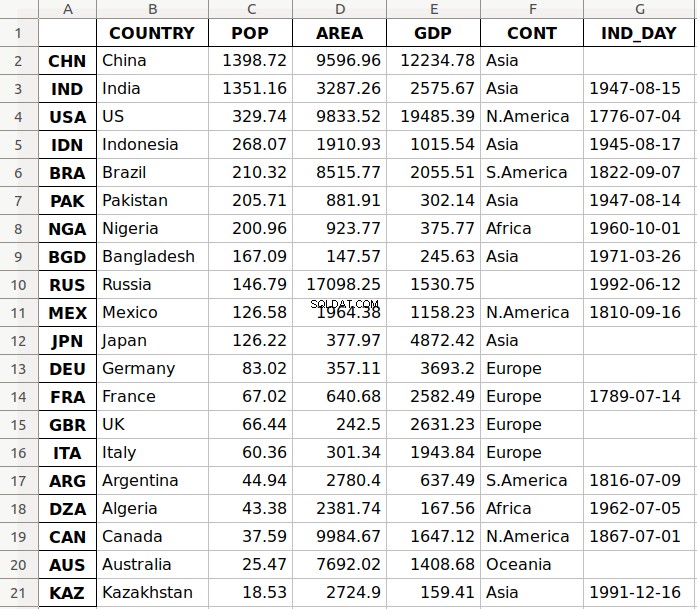
>>> df.to_sql('data.db', con=engine, index_label='ID')
The parameter con is used to specify the database connection or engine that you want to use. The optional parameter index_label specifies how to call the database column with the row labels. You’ll often see it take on the value ID , Id , or id .
You should get the database data.db with a single table that looks like this:
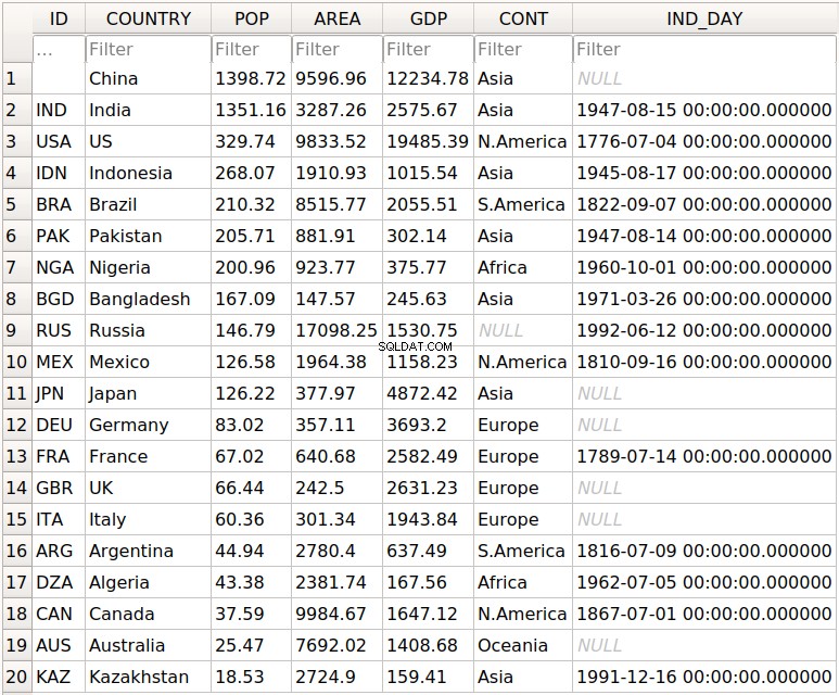
The first column contains the row labels. To omit writing them into the database, pass index=False to .to_sql() . The other columns correspond to the columns of the DataFrame .
There are a few more optional parameters. For example, you can use schema to specify the database schema and dtype to determine the types of the database columns. You can also use if_exists , which says what to do if a database with the same name and path already exists:
if_exists='fail'raises a ValueError and is the default.if_exists='replace'drops the table and inserts new values.if_exists='append'inserts new values into the table.
You can load the data from the database with read_sql() :
>>> df = pd.read_sql('data.db', con=engine, index_col='ID')
>>> df
        COUNTRY      POP      AREA       GDP       CONT    IND_DAY
ID
CHN       China  1398.72   9596.96  12234.78       Asia        NaT
IND       India  1351.16   3287.26   2575.67       Asia 1947-08-15
USA          US   329.74   9833.52  19485.39  N.America 1776-07-04
IDN   Indonesia   268.07   1910.93   1015.54       Asia 1945-08-17
BRA      Brazil   210.32   8515.77   2055.51  S.America 1822-09-07
PAK    Pakistan   205.71    881.91    302.14       Asia 1947-08-14
NGA     Nigeria   200.96    923.77    375.77     Africa 1960-10-01
BGD  Bangladesh   167.09    147.57    245.63       Asia 1971-03-26
RUS      Russia   146.79  17098.25   1530.75       None 1992-06-12
MEX      Mexico   126.58   1964.38   1158.23  N.America 1810-09-16
JPN       Japan   126.22    377.97   4872.42       Asia        NaT
DEU     Germany    83.02    357.11   3693.20     Europe        NaT
FRA      France    67.02    640.68   2582.49     Europe 1789-07-14
GBR          UK    66.44    242.50   2631.23     Europe        NaT
ITA       Italy    60.36    301.34   1943.84     Europe        NaT
ARG   Argentina    44.94   2780.40    637.49  S.America 1816-07-09
DZA     Algeria    43.38   2381.74    167.56     Africa 1962-07-05
CAN      Canada    37.59   9984.67   1647.12  N.America 1867-07-01
AUS   Australia    25.47   7692.02   1408.68    Oceania        NaT
KAZ  Kazakhstan    18.53   2724.90    159.41       Asia 1991-12-16
The parameter index_col specifies the name of the column with the row labels. Note that this inserts an extra row after the header that starts with ID . You can fix this behavior with the following line of code:
>>> df.index.name = None
>>> df
        COUNTRY      POP      AREA       GDP       CONT    IND_DAY
CHN       China  1398.72   9596.96  12234.78       Asia        NaT
IND       India  1351.16   3287.26   2575.67       Asia 1947-08-15
USA          US   329.74   9833.52  19485.39  N.America 1776-07-04
IDN   Indonesia   268.07   1910.93   1015.54       Asia 1945-08-17
BRA      Brazil   210.32   8515.77   2055.51  S.America 1822-09-07
PAK    Pakistan   205.71    881.91    302.14       Asia 1947-08-14
NGA     Nigeria   200.96    923.77    375.77     Africa 1960-10-01
BGD  Bangladesh   167.09    147.57    245.63       Asia 1971-03-26
RUS      Russia   146.79  17098.25   1530.75       None 1992-06-12
MEX      Mexico   126.58   1964.38   1158.23  N.America 1810-09-16
JPN       Japan   126.22    377.97   4872.42       Asia        NaT
DEU     Germany    83.02    357.11   3693.20     Europe        NaT
FRA      France    67.02    640.68   2582.49     Europe 1789-07-14
GBR          UK    66.44    242.50   2631.23     Europe        NaT
ITA       Italy    60.36    301.34   1943.84     Europe        NaT
ARG   Argentina    44.94   2780.40    637.49  S.America 1816-07-09
DZA     Algeria    43.38   2381.74    167.56     Africa 1962-07-05
CAN      Canada    37.59   9984.67   1647.12  N.America 1867-07-01
AUS   Australia    25.47   7692.02   1408.68    Oceania        NaT
KAZ  Kazakhstan    18.53   2724.90    159.41       Asia 1991-12-16
Now you have the same DataFrame object as before.
Note that the continent for Russia is now None instead of nan . If you want to fill the missing values with nan , then you can use .fillna() :
>>> df.fillna(value=float('nan'), inplace=True)
.fillna() replaces all missing values with whatever you pass to value . Here, you passed float('nan') , which says to fill all missing values with nan .
Also note that you didn’t have to pass parse_dates=['IND_DAY'] to read_sql() . That’s because your database was able to detect that the last column contains dates. However, you can pass parse_dates jika Anda mau. You’ll get the same results.
There are other functions that you can use to read databases, like read_sql_table() and read_sql_query() . Feel free to try them out!
Pickle Files
Pickling is the act of converting Python objects into byte streams. Unpickling is the inverse process. Python pickle files are the binary files that keep the data and hierarchy of Python objects. They usually have the extension .pickle or .pkl .
You can save your DataFrame in a pickle file with .to_pickle() :
>>> dtypes = {'POP': 'float64', 'AREA': 'float64', 'GDP': 'float64',
...           'IND_DAY': 'datetime64'}
>>> df = pd.DataFrame(data=data).T.astype(dtype=dtypes)
>>> df.to_pickle('data.pickle')
Like you did with databases, it can be convenient first to specify the data types. Then, you create a file data.pickle to contain your data. You could also pass an integer value to the optional parameter protocol , which specifies the protocol of the pickler.
You can get the data from a pickle file with read_pickle() :
>>> df = pd.read_pickle('data.pickle')
>>> df
        COUNTRY      POP      AREA       GDP       CONT    IND_DAY
CHN       China  1398.72   9596.96  12234.78       Asia        NaT
IND       India  1351.16   3287.26   2575.67       Asia 1947-08-15
USA          US   329.74   9833.52  19485.39  N.America 1776-07-04
IDN   Indonesia   268.07   1910.93   1015.54       Asia 1945-08-17
BRA      Brazil   210.32   8515.77   2055.51  S.America 1822-09-07
PAK    Pakistan   205.71    881.91    302.14       Asia 1947-08-14
NGA     Nigeria   200.96    923.77    375.77     Africa 1960-10-01
BGD  Bangladesh   167.09    147.57    245.63       Asia 1971-03-26
RUS      Russia   146.79  17098.25   1530.75        NaN 1992-06-12
MEX      Mexico   126.58   1964.38   1158.23  N.America 1810-09-16
JPN       Japan   126.22    377.97   4872.42       Asia        NaT
DEU     Germany    83.02    357.11   3693.20     Europe        NaT
FRA      France    67.02    640.68   2582.49     Europe 1789-07-14
GBR          UK    66.44    242.50   2631.23     Europe        NaT
ITA       Italy    60.36    301.34   1943.84     Europe        NaT
ARG   Argentina    44.94   2780.40    637.49  S.America 1816-07-09
DZA     Algeria    43.38   2381.74    167.56     Africa 1962-07-05
CAN      Canada    37.59   9984.67   1647.12  N.America 1867-07-01
AUS   Australia    25.47   7692.02   1408.68    Oceania        NaT
KAZ  Kazakhstan    18.53   2724.90    159.41       Asia 1991-12-16
read_pickle() returns the DataFrame with the stored data. You can also check the data types:
>>> df.dtypes
COUNTRY            object
POP               float64
AREA              float64
GDP               float64
CONT               object
IND_DAY    datetime64[ns]
dtype: object
These are the same ones that you specified before using .to_pickle() .
As a word of caution, you should always beware of loading pickles from untrusted sources. This can be dangerous! When you unpickle an untrustworthy file, it could execute arbitrary code on your machine, gain remote access to your computer, or otherwise exploit your device in other ways.
Working With Big Data
If your files are too large for saving or processing, then there are several approaches you can take to reduce the required disk space:
- Compress your files
- Choose only the columns you want
- Omit the rows you don’t need
- Force the use of less precise data types
- Split the data into chunks
You’ll take a look at each of these techniques in turn.
Compress and Decompress Files
You can create an archive file like you would a regular one, with the addition of a suffix that corresponds to the desired compression type:
'.gz''.bz2''.zip''.xz'
Pandas can deduce the compression type by itself:
>>>>>> df = pd.DataFrame(data=data).T
>>> df.to_csv('data.csv.zip')
Here, you create a compressed .csv file as an archive. The size of the regular .csv file is 1048 bytes, while the compressed file only has 766 bytes.
You can open this compressed file as usual with the Pandas read_csv() function:
>>> df = pd.read_csv('data.csv.zip', index_col=0,
...                  parse_dates=['IND_DAY'])
>>> df
        COUNTRY      POP      AREA       GDP       CONT    IND_DAY
CHN       China  1398.72   9596.96  12234.78       Asia        NaT
IND       India  1351.16   3287.26   2575.67       Asia 1947-08-15
USA          US   329.74   9833.52  19485.39  N.America 1776-07-04
IDN   Indonesia   268.07   1910.93   1015.54       Asia 1945-08-17
BRA      Brazil   210.32   8515.77   2055.51  S.America 1822-09-07
PAK    Pakistan   205.71    881.91    302.14       Asia 1947-08-14
NGA     Nigeria   200.96    923.77    375.77     Africa 1960-10-01
BGD  Bangladesh   167.09    147.57    245.63       Asia 1971-03-26
RUS      Russia   146.79  17098.25   1530.75        NaN 1992-06-12
MEX      Mexico   126.58   1964.38   1158.23  N.America 1810-09-16
JPN       Japan   126.22    377.97   4872.42       Asia        NaT
DEU     Germany    83.02    357.11   3693.20     Europe        NaT
FRA      France    67.02    640.68   2582.49     Europe 1789-07-14
GBR          UK    66.44    242.50   2631.23     Europe        NaT
ITA       Italy    60.36    301.34   1943.84     Europe        NaT
ARG   Argentina    44.94   2780.40    637.49  S.America 1816-07-09
DZA     Algeria    43.38   2381.74    167.56     Africa 1962-07-05
CAN      Canada    37.59   9984.67   1647.12  N.America 1867-07-01
AUS   Australia    25.47   7692.02   1408.68    Oceania        NaT
KAZ  Kazakhstan    18.53   2724.90    159.41       Asia 1991-12-16
read_csv() decompresses the file before reading it into a DataFrame .
You can specify the type of compression with the optional parameter compression , which can take on any of the following values:
'infer''gzip''bz2''zip''xz'None
The default value compression='infer' indicates that Pandas should deduce the compression type from the file extension.
Here’s how you would compress a pickle file:
>>>>>> df = pd.DataFrame(data=data).T
>>> df.to_pickle('data.pickle.compress', compression='gzip')
You should get the file data.pickle.compress that you can later decompress and read:
>>> df = pd.read_pickle('data.pickle.compress', compression='gzip')
df again corresponds to the DataFrame with the same data as before.
You can give the other compression methods a try, as well. If you’re using pickle files, then keep in mind that the .zip format supports reading only.
Choose Columns
The Pandas read_csv() and read_excel() functions have the optional parameter usecols that you can use to specify the columns you want to load from the file. You can pass the list of column names as the corresponding argument:
>>> df = pd.read_csv('data.csv', usecols=['COUNTRY', 'AREA'])
>>> df
       COUNTRY      AREA
0        China   9596.96
1        India   3287.26
2           US   9833.52
3    Indonesia   1910.93
4       Brazil   8515.77
5     Pakistan    881.91
6      Nigeria    923.77
7   Bangladesh    147.57
8       Russia  17098.25
9       Mexico   1964.38
10       Japan    377.97
11     Germany    357.11
12      France    640.68
13          UK    242.50
14       Italy    301.34
15   Argentina   2780.40
16     Algeria   2381.74
17      Canada   9984.67
18   Australia   7692.02
19  Kazakhstan   2724.90
Now you have a DataFrame that contains less data than before. Here, there are only the names of the countries and their areas.
Instead of the column names, you can also pass their indices:
>>>>>> df = pd.read_csv('data.csv',index_col=0, usecols=[0, 1, 3])
>>> df
COUNTRY AREA
CHN China 9596.96
IND India 3287.26
USA US 9833.52
IDN Indonesia 1910.93
BRA Brazil 8515.77
PAK Pakistan 881.91
NGA Nigeria 923.77
BGD Bangladesh 147.57
RUS Russia 17098.25
MEX Mexico 1964.38
JPN Japan 377.97
DEU Germany 357.11
FRA France 640.68
GBR UK 242.50
ITA Italy 301.34
ARG Argentina 2780.40
DZA Algeria 2381.74
CAN Canada 9984.67
AUS Australia 7692.02
KAZ Kazakhstan 2724.90
Expand the code block below to compare these results with the file 'data.csv' :
,COUNTRY,POP,AREA,GDP,CONT,IND_DAY
CHN,China,1398.72,9596.96,12234.78,Asia,
IND,India,1351.16,3287.26,2575.67,Asia,1947-08-15
USA,US,329.74,9833.52,19485.39,N.America,1776-07-04
IDN,Indonesia,268.07,1910.93,1015.54,Asia,1945-08-17
BRA,Brazil,210.32,8515.77,2055.51,S.America,1822-09-07
PAK,Pakistan,205.71,881.91,302.14,Asia,1947-08-14
NGA,Nigeria,200.96,923.77,375.77,Africa,1960-10-01
BGD,Bangladesh,167.09,147.57,245.63,Asia,1971-03-26
RUS,Russia,146.79,17098.25,1530.75,,1992-06-12
MEX,Mexico,126.58,1964.38,1158.23,N.America,1810-09-16
JPN,Japan,126.22,377.97,4872.42,Asia,
DEU,Germany,83.02,357.11,3693.2,Europe,
FRA,France,67.02,640.68,2582.49,Europe,1789-07-14
GBR,UK,66.44,242.5,2631.23,Europe,
ITA,Italy,60.36,301.34,1943.84,Europe,
ARG,Argentina,44.94,2780.4,637.49,S.America,1816-07-09
DZA,Algeria,43.38,2381.74,167.56,Africa,1962-07-05
CAN,Canada,37.59,9984.67,1647.12,N.America,1867-07-01
AUS,Australia,25.47,7692.02,1408.68,Oceania,
KAZ,Kazakhstan,18.53,2724.9,159.41,Asia,1991-12-16
You can see the following columns:
- The column at index
0contains the row labels. - The column at index
1contains the country names. - The column at index
3contains the areas.
Simlarly, read_sql() has the optional parameter columns that takes a list of column names to read:
>>> df = pd.read_sql('data.db', con=engine, index_col='ID',
...                  columns=['COUNTRY', 'AREA'])
>>> df.index.name = None
>>> df
        COUNTRY      AREA
CHN       China   9596.96
IND       India   3287.26
USA          US   9833.52
IDN   Indonesia   1910.93
BRA      Brazil   8515.77
PAK    Pakistan    881.91
NGA     Nigeria    923.77
BGD  Bangladesh    147.57
RUS      Russia  17098.25
MEX      Mexico   1964.38
JPN       Japan    377.97
DEU     Germany    357.11
FRA      France    640.68
GBR          UK    242.50
ITA       Italy    301.34
ARG   Argentina   2780.40
DZA     Algeria   2381.74
CAN      Canada   9984.67
AUS   Australia   7692.02
KAZ  Kazakhstan   2724.90
Again, the DataFrame only contains the columns with the names of the countries and areas. If columns is None or omitted, then all of the columns will be read, as you saw before. The default behavior is columns=None .
Omit Rows
When you test an algorithm for data processing or machine learning, you often don’t need the entire dataset. It’s convenient to load only a subset of the data to speed up the process. The Pandas read_csv() and read_excel() functions have some optional parameters that allow you to select which rows you want to load:
skiprows: either the number of rows to skip at the beginning of the file if it’s an integer, or the zero-based indices of the rows to skip if it’s a list-like objectskipfooter: the number of rows to skip at the end of the filenrows: the number of rows to read
Here’s how you would skip rows with odd zero-based indices, keeping the even ones:
>>>>>> df = pd.read_csv('data.csv', index_col=0, skiprows=range(1, 20, 2))
>>> df
COUNTRY POP AREA GDP CONT IND_DAY
IND India 1351.16 3287.26 2575.67 Asia 1947-08-15
IDN Indonesia 268.07 1910.93 1015.54 Asia 1945-08-17
PAK Pakistan 205.71 881.91 302.14 Asia 1947-08-14
BGD Bangladesh 167.09 147.57 245.63 Asia 1971-03-26
MEX Mexico 126.58 1964.38 1158.23 N.America 1810-09-16
DEU Germany 83.02 357.11 3693.20 Europe NaN
GBR UK 66.44 242.50 2631.23 Europe NaN
ARG Argentina 44.94 2780.40 637.49 S.America 1816-07-09
CAN Canada 37.59 9984.67 1647.12 N.America 1867-07-01
KAZ Kazakhstan 18.53 2724.90 159.41 Asia 1991-12-16
In this example, skiprows is range(1, 20, 2) and corresponds to the values 1 , 3 , …, 19 . The instances of the Python built-in class range behave like sequences. The first row of the file data.csv is the header row. It has the index 0 , so Pandas loads it in. The second row with index 1 corresponds to the label CHN , and Pandas skips it. The third row with the index 2 and label IND is loaded, and so on.
If you want to choose rows randomly, then skiprows can be a list or NumPy array with pseudo-random numbers, obtained either with pure Python or with NumPy.
Force Less Precise Data Types
If you’re okay with less precise data types, then you can potentially save a significant amount of memory! First, get the data types with .dtypes again:
>>> df = pd.read_csv('data.csv', index_col=0, parse_dates=['IND_DAY'])
>>> df.dtypes
COUNTRY            object
POP               float64
AREA              float64
GDP               float64
CONT               object
IND_DAY    datetime64[ns]
dtype: object
The columns with the floating-point numbers are 64-bit floats. Each number of this type float64 consumes 64 bits or 8 bytes. Each column has 20 numbers and requires 160 bytes. You can verify this with .memory_usage() :
>>> df.memory_usage()
Index      160
COUNTRY    160
POP        160
AREA       160
GDP        160
CONT       160
IND_DAY    160
dtype: int64
.memory_usage() returns an instance of Series with the memory usage of each column in bytes. You can conveniently combine it with .loc[] and .sum() to get the memory for a group of columns:
>>> df.loc[:, ['POP', 'AREA', 'GDP']].memory_usage(index=False).sum()
480
This example shows how you can combine the numeric columns 'POP' , 'AREA' , and 'GDP' to get their total memory requirement. The argument index=False excludes data for row labels from the resulting Series object. For these three columns, you’ll need 480 bytes.
You can also extract the data values in the form of a NumPy array with .to_numpy() or .values . Then, use the .nbytes attribute to get the total bytes consumed by the items of the array:
>>> df.loc[:, ['POP', 'AREA', 'GDP']].to_numpy().nbytes
480
The result is the same 480 bytes. So, how do you save memory?
In this case, you can specify that your numeric columns 'POP' , 'AREA' , and 'GDP' should have the type float32 . Use the optional parameter dtype to do this:
>>> dtypes = {'POP': 'float32', 'AREA': 'float32', 'GDP': 'float32'}
>>> df = pd.read_csv('data.csv', index_col=0, dtype=dtypes,
...                  parse_dates=['IND_DAY'])
The dictionary dtypes specifies the desired data types for each column. It’s passed to the Pandas read_csv() function as the argument that corresponds to the parameter dtype .
Now you can verify that each numeric column needs 80 bytes, or 4 bytes per item:
>>>>>> df.dtypes
COUNTRY object
POP float32
AREA float32
GDP float32
CONT object
IND_DAY datetime64[ns]
dtype: object
>>> df.memory_usage()
Index 160
COUNTRY 160
POP 80
AREA 80
GDP 80
CONT 160
IND_DAY 160
dtype: int64
>>> df.loc[:, ['POP', 'AREA', 'GDP']].memory_usage(index=False).sum()
240
>>> df.loc[:, ['POP', 'AREA', 'GDP']].to_numpy().nbytes
240
Each value is a floating-point number of 32 bits or 4 bytes. The three numeric columns contain 20 items each. In total, you’ll need 240 bytes of memory when you work with the type float32 . This is half the size of the 480 bytes you’d need to work with float64 .
In addition to saving memory, you can significantly reduce the time required to process data by using float32 instead of float64 in some cases.
Use Chunks to Iterate Through Files
Another way to deal with very large datasets is to split the data into smaller chunks and process one chunk at a time. If you use read_csv() , read_json() or read_sql() , then you can specify the optional parameter chunksize :
>>> data_chunk = pd.read_csv('data.csv', index_col=0, chunksize=8)
>>> type(data_chunk)
<class 'pandas.io.parsers.TextFileReader'>
>>> hasattr(data_chunk, '__iter__')
True
>>> hasattr(data_chunk, '__next__')
True
chunksize defaults to None and can take on an integer value that indicates the number of items in a single chunk. When chunksize is an integer, read_csv() returns an iterable that you can use in a for loop to get and process only a fragment of the dataset in each iteration:
>>> for df_chunk in pd.read_csv('data.csv', index_col=0, chunksize=8):
...     print(df_chunk, end='\n\n')
...     print('memory:', df_chunk.memory_usage().sum(), 'bytes',
...           end='\n\n\n')
...
        COUNTRY      POP     AREA       GDP       CONT     IND_DAY
CHN       China  1398.72  9596.96  12234.78       Asia         NaN
IND       India  1351.16  3287.26   2575.67       Asia  1947-08-15
USA          US   329.74  9833.52  19485.39  N.America  1776-07-04
IDN   Indonesia   268.07  1910.93   1015.54       Asia  1945-08-17
BRA      Brazil   210.32  8515.77   2055.51  S.America  1822-09-07
PAK    Pakistan   205.71   881.91    302.14       Asia  1947-08-14
NGA     Nigeria   200.96   923.77    375.77     Africa  1960-10-01
BGD  Bangladesh   167.09   147.57    245.63       Asia  1971-03-26

memory: 448 bytes


       COUNTRY     POP      AREA      GDP       CONT     IND_DAY
RUS     Russia  146.79  17098.25  1530.75        NaN  1992-06-12
MEX     Mexico  126.58   1964.38  1158.23  N.America  1810-09-16
JPN      Japan  126.22    377.97  4872.42       Asia         NaN
DEU    Germany   83.02    357.11  3693.20     Europe         NaN
FRA     France   67.02    640.68  2582.49     Europe  1789-07-14
GBR         UK   66.44    242.50  2631.23     Europe         NaN
ITA      Italy   60.36    301.34  1943.84     Europe         NaN
ARG  Argentina   44.94   2780.40   637.49  S.America  1816-07-09

memory: 448 bytes


        COUNTRY    POP     AREA      GDP       CONT     IND_DAY
DZA     Algeria  43.38  2381.74   167.56     Africa  1962-07-05
CAN      Canada  37.59  9984.67  1647.12  N.America  1867-07-01
AUS   Australia  25.47  7692.02  1408.68    Oceania         NaN
KAZ  Kazakhstan  18.53  2724.90   159.41       Asia  1991-12-16

memory: 224 bytes
In this example, the chunksize is 8 . The first iteration of the for loop returns a DataFrame with the first eight rows of the dataset only. The second iteration returns another DataFrame with the next eight rows. The third and last iteration returns the remaining four rows.
Catatan: You can also pass iterator=True to force the Pandas read_csv() function to return an iterator object instead of a DataFrame object.
In each iteration, you get and process the DataFrame with the number of rows equal to chunksize . It’s possible to have fewer rows than the value of chunksize in the last iteration. You can use this functionality to control the amount of memory required to process data and keep that amount reasonably small.
Kesimpulan
You now know how to save the data and labels from Pandas DataFrame objects to different kinds of files. You also know how to load your data from files and create DataFrame objects.
You’ve used the Pandas read_csv() and .to_csv() methods to read and write CSV files. You also used similar methods to read and write Excel, JSON, HTML, SQL, and pickle files. These functions are very convenient and widely used. They allow you to save or load your data in a single function or method call.
You’ve also learned how to save time, memory, and disk space when working with large data files:
- Compress or decompress files
- Choose the rows and columns you want to load
- Use less precise data types
- Split data into chunks and process them one by one
You’ve mastered a significant step in the machine learning and data science process! If you have any questions or comments, then please put them in the comments section below.